All of the code for this workshop is available on GitHub. We encourage you to play around with the examples as you follow along.
Bayesian inference gives us a recipe for optimally revising uncertain beliefs after receiving evidence. Often times, we have good models of how hidden states of the world produce different outcomes, but we want to know what those hidden states are. Bayes’ rule gives us a recipe for solving such inverse problems.
Consider our remarkable ability to infer what’s going on in other people’s minds. When a friend seems to be acting unusually cold or irritable, we can effortlessly conjure up a number of hypotheses about the cause of this behavior. Maybe my friend is angry with me, maybe he didn’t sleep well, maybe he’s hungry, and so on. We can do this because we have a model of how different behaviors are produced by different mental causes. I might know that when my friend is angry, he is likely to act passive aggressively, while this behavior is rare when he is happy. With a model of how observable behavior is produced by various possible hidden causes — along with baseline beliefs about the plausibility of these different causes — we can help identify the particular cause of the behavior at hand.
Bayes’ theorem also gives us an elegant way to estimate coefficients in statistical models (e.g., linear regression). We’ll tackle this problem in the second part of the workshop.
Toy Examples
Here we present three toy models to help explain the basic mechanics of Bayes’ theorem. Code for the chocolate model and email model are available in separate files.
Coin flips
Most tutorials on probability theory and Bayesian reasoning begin with an analysis of coin flips because they are one of the simplest systems to work with. Imagine that we observe a sequence of flips of heads (\(H\)) or tails (\(T\)). We want to infer the probability \(p\) that the coin will land heads on a given flip.
Although this may be a simple example for people familiar with the topic, let’s be concrete about the exact inference problem at hand. What is unknown? In this case, it is a particular state of the coin: its probability of landing heads, which can take on any value from 0 (coin always lands tails) to 1 (coin always lands heads). Thus, for any probability \(p\) such that \(0 \leq p \leq 1\), we want to know how confident we should be that the coin lands heads with this probability.
At this point, it’s easy to get confused, as our confidence is itself probabilistic. That is, we are assigning a probability to a probability that the coin lands heads. But these probabilities are distinct: the former represents our subjective credence in the latter, which is a state of the coin. The former is what Bayes’ theorem updates.
For each \(p\), we start with a prior belief that the coin lands heads with that probability:
\[P(\text{coin lands heads with probability } p).\]
After observing some data (a sequence of coin flips), we end up with a new belief, known as the posterior:
\[P(\text{coin lands heads with probability } p | D),\]
where \(D\) is the data and the “|” reads as “given.”
How do we correctly incorporate this new data into our beliefs? We must first build a model of how this data could be produced from the unknown parameters we’re trying to estimate (in this case \(p\)). This model specifies the probability of obtaining our data given different parameter values. This quantity, known as the likelihood, is generally the most challenging quantity to calculate and is often the only thing that orthodox statistical methods care about. For example, the method of maximum likelihood estimation (MLE) would identity the value of \(p\) that maximizes
\[P(D | \text{coin lands heads with probability } p).\]
But Bayesians rightfully point out that the likelihood is not the quantity we ultimately care about. Imagine, for instance, that you’ve just observed two heads in a row from this unknown coin (\(D=H_1H_2\)). The likelihood of observing this data is \(p*p=p^2\). It is easy to see that this quantity is maximized when \(p=1\), i.e., when the coin is rigged to always land heads. Most of us would not jump to this conclusion, though. Clearly, our prior belief that almost all coins in the world land heads with 50% probability exerts a large pull on our beliefs, especially in a case like this, in which data is limited.
That brings us to the crux of Bayes’ theorem, which gives us an easy way to integrate the prior and likelihood into the posterior. All you do is multiply:
\[posterior \propto prior*likelihood.\]
We use the “\(\propto\)” symbol here to indicate that the posterior is proportional to the product of the prior and likelihood up to a normalizing constant. In practice, this is usually all that we’ll need.
Now let’s come back to our example with \(D=H_1H_2\). As we saw above, the likelihood in this case is just \(p^2\). But to get posterior beliefs for different \(p\) values, we need to specify a prior over the plausibility of these \(p\) values. Here’s a simple one: assume with 95% probability that the coin is fair (\(p=.5\)) and with the remaining 5% probability that the coin is fully rigged to always give heads or always give tails. That is,
\[P(\text{coin lands heads with probability } .5) = .95,\] \[P(\text{coin lands heads with probability } 1) = .025,\] and
\[P(\text{coin lands heads with probability } 0) = .025.\]
Assign the prior probability for any other \(p\) to 0.
From Bayes’ theorem, we can already see that we can discount any value of \(p\) other than 0, .5, and 1, as the prior will be 0 and, therefore, the product of the prior and likelihood will yield a posterior of 0. This means we only need to evaluate the three cases where \(p\) is 0, .5, or 1. Multiplying the priors from above with the likelihoods, we get (unnormalized) posteriors of \(.025*0^2\), \(.95*.5^2\), and \(.025*1^2\), respectively. (If we wanted to turn these quantities into probabilities that sum to 1, we could divide each term by the sum of all terms.) Clearly, the posterior for \(p=.5\) (.238) is much larger than the posterior for \(p=1\) (.025) and \(p=0\) (0), matching our intuition that observing two heads from an unknown coin is insufficient evidence to overcome our prior belief that the coin is fair. Indeed, \(p=.5\) is the maximum a posteriori (MAP) estimate: the value that we deem most probable after observing the data.
Beta binomial model
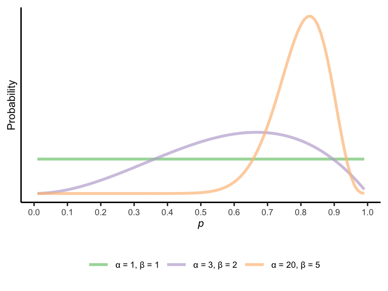
Sometimes we can write out our prior in a way that greatly simplifies the math of Bayes’ theorem and doesn’t require computing posteriors separately for each possible \(p\) value. In the case of estimating the probability of a coin’s landing heads — or estimating other probabilities with this structure, such as the probability that a candidate will get a vote in a two-person election, the probability that somebody in our in-group will agree with a policy position, and so on — it is common to use a beta distribution as the prior. This distribution has two positive shape parameters, \(\alpha\) and \(\beta\), which weigh the relative plausibility of high and low \(p\) values, respectively.1 See below for some examples.
Now suppose that your data consists of observing \(k\) heads out of \(n\) coin flips. If your prior is beta-distributed with shape parameters \(\alpha\) and \(\beta\), then your posterior will also be beta-distributed, with shape parameters \(\alpha + k\) and \(\beta + (n - k)\). In other words, we can simply add the counts of heads and tails to our prior \(\alpha\) and \(\beta\) parameters, respectively.
This is a powerful trick, which you’ll see exploited in many Bayesian models. Bear in mind, though, that there are many priors that cannot be represented with a beta distribution, such as the example we used above where we assigned 0 prior probability to almost all \(p\) values.
How much does Adam like chocolate cake?
Let’s switch gears to a more complicated example: reading minds. Or at least reading one tiny facet of a person’s mind, which is their preference for a tasty dessert.
Imagine you have the following information. Adam is generally indifferent about eating non-chocolate desserts, but he has a sweet tooth for chocolate. Unfortunately, he’s also lactose intolerant, which makes him averse to eating most foods with lactose when he doesn’t have his Lactaid pills on him. He is occasionally willing to eat foods with lactose if he absolutely loves them, but you’re not sure if chocolate desserts meet this threshold. (Assume for the sake of this simple example that there’s no correlation between a dessert’s containing chocolate and its containing lactose and also that the amount of lactose in desserts is all or none.)
Now you’re out to dinner with Adam, who has pointed out that he forgot to bring Lactaid with him this evening. You run to the bathroom, and when you return, you see Adam zealously eating a chocolate dessert. You don’t know whether the dessert contains lactose, but Adam does. What do you infer about the dessert’s lactose content and Adam’s love of chocolate desserts?
Before delving into the math of this silly example, just take a moment to think intuitively about how your beliefs might change after seeing Adam eat the dessert. Two things were initially unknown: (a) whether the dessert contains lactose and (b) how much Adam loves chocolate desserts. Presumably, if you initially thought the dessert might contain lactose, you’re less likely to believe this now, since you know that Adam generally avoids foods containing lactose. At the same time, you remain open to the possibility that Adam just loves chocolate desserts so much that he was willing to incur the cost of digestive issues to enjoy this particular dessert. So, after seeing Adam eat the dessert, you simultaneously believe that it is less likely to contain lactose and more desirable to him.
How might we formalize this? It’s first worth stressing that there’s almost never a ‘correct’ way of doing this, and any model is necessarily going to have to make certain simplifying assumptions. So as we walk through this particular formalization, think about how you might tweak certain details or build in more structure. And, most importantly, think about how you could make the example more realistic to apply it to a real research problem.
In general, for models of decision-making, it’s standard to imagine that the decision-maker assigns some scalar utility to different actions based on their features. By convention, the actor wants to act when the utility is positive and doesn’t want to act when the utility is negative. Now recall, “Adam is generally indifferent about eating non-chocolate desserts.” This is a useful (and unrealistic) clue that Adam assigns a utility of 0 to non-chocolate desserts. Meanwhile, we are told that Adam likes chocolate, suggesting that his utility from eating such a dessert is positive on its own. However, we are also told that Adam finds foods containing lactose to be aversive, suggesting that lactose lowers a food’s utility. Putting it all together, we can write Adam’s utility \(U\) for eating desserts as
\[U = b_cC - b_lL,\]
where \(C\) and \(L\) are binary values set to 1 if the dessert contains chocolate and lactose, respectively, and \(b_c\) and \(b_l\) indicate the respective dis(utility) from eating a dessert with chocolate and lactose. For simplicity, we can set \(b_l\) to 1, since really what we care about is Adam’s love of chocolate relative to his discomfort from eating food with lactose. Therefore, the scale is arbitrary, and when \(b_l=1\), \(b_c\) tells us how Adam’s love of chocolate compares to his hatred for lactose. If \(b_c=1\), they are exactly equal, and Adam is indifferent about eating a chocolate dessert with lactose. If \(b_c>1\), Adam is willing to eat the dessert despite having lactose, and vice versa for \(b_c<1\). Also notice that \(U=0\) for non-chocolate desserts (that don’t contain lactose), correctly indicating that Adam is indifferent about eating such desserts.
Now that we have this utility model written down, we need to convert this to a likelihood function that Bayes’ theorem can work with. Our “data” in this case is our observation of Adam’s eating a chocolate dessert. What’s unknown is how much Adam loves chocolate desserts (\(b_c\)) and whether the dessert contains lactose (\(L\)). Thus, we need an expression for
\[P(D=\text{Adam eats chocolate dessert}|b_c,L).\]
We could simply set this probability to 1 when \(U>0\), 0 when \(U<0\), and .5 when \(U=0\). But the real world is messy, and there are many unmodeled factors that likely add noise to Adam’s decision to eat or not eat desserts (e.g., he might be more or less full from the dinner he just ate). Thus, to translate utilities into action probabilities, it is typical to pass the utility to a logistic function. (Does the word “logistic” ring any bells?) In essence, this function will map \(U\) values near 0 to approximately .5 and gradually increase the output toward a probability of 1 as \(U\) increases further (and vice versa as it decreases below \(U=0\)). The function takes a single parameter that controls the steepness of the transition. As you can see in the code, we choose a relatively steep curve, but you can play around with this setting yourself to see how it affects the results.
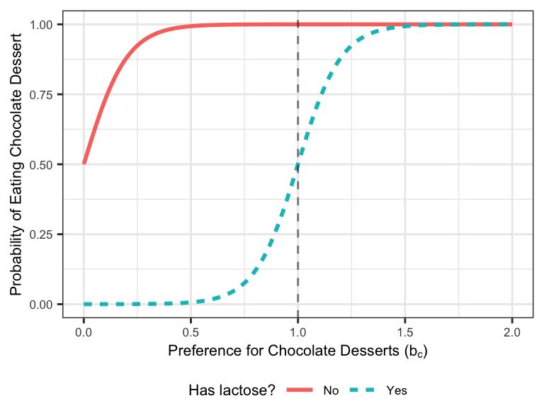
In short, with \(b_l=1\) and \(C=1\) (indicating that the dessert is chocolate), the utility function of Adam eating a chocolate dessert reduces to \(b_c - L\). Thus, the likelihood becomes
\[P(D|b_c,L) = \text{logistic}(b_c-L).\]
Let’s take a look at this function below. The probability of Adam’s eating chocolate dessert based on his preference for chocolate has the characteristic “S” shape of the logistic function. However, this curve is shifted 1 unit to the right when the dessert contains lactose (dashed line), indicating that Adam’s indifference point occurs when \(b_c=1\), i.e., when his preference for chocolate perfectly compensates for his aversion to lactose.
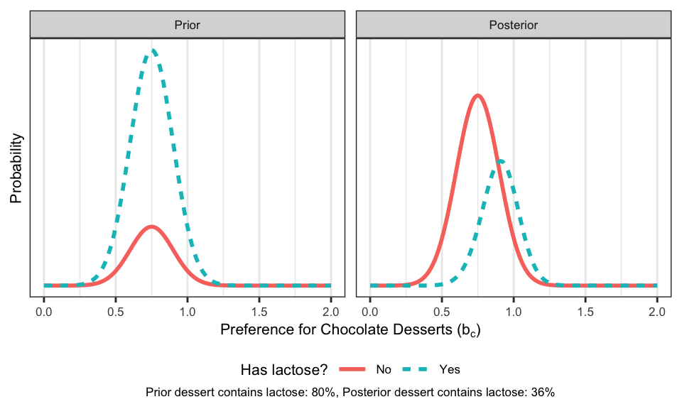
So far so good. Now let’s estimate what we really want: the posterior, \(P(b_c,L|D)\). To do this, we first need to specify a prior, \(P(b_c,L)\). Because we are jointly estimating two variables, this prior is 2-dimensional. However, if we believe that Adam’s love of chocolate and the probability that the dessert has lactose are uncorrelated, we can decompose the prior into the product of the two individual terms: \(P(b_c)P(L)\). For the sake of space, we won’t go into detail here about how this prior is specified and instead simply show one example below. (As always, we encourage you to play around with the code!) In this example, we start with a relatively strong belief that the chocolate dessert contains lactose, and our prior on Adam’s love of chocolate desserts is centered a little below 1 (left panel). That is, we start off believing that Adam is unlikely to like chocolate enough to eat a chocolate dessert that contains lactose. However, we remain open to the possibility that \(b_c > 1\).
What happens after we observe Adam eat the chocolate dessert? Multiplying the prior by the likelihood to get a posterior, we see a shift in our beliefs in both of the directions that we intuitively predicted. Now we believe that the dessert is unlikely to contain lactose, but we also believe it’s possible that it contains lactose but that Adam loves chocolate more than we initially thought (right panel).
It’s worth pointing out one final quirk about this update. Recall that before we observed Adam eat the dessert, we assumed that whether the dessert has lactose and how much Adam loves chocolate were uncorrelated. But after gathering our data, these two variables have become correlated. If, for example, Adam tells us that the dessert contains lactose, this gives us information about how much he loves chocolate desserts (a lot!). Likewise, if Adam tells us he loves chocolate so much that he’s willing to get sick, this gives us information about the probability that the dessert contains lactose. This is a cool example of a collider.
Ben’s favo(u)rite professor
Ben has a favorite professor, who he’s been too afraid to email. One day, he works up the courage to finally send that email, hopeful that he’ll receive an encouraging reply. As each day passes without a reply, though, Ben begins to wonder whether he’ll ever hear back. He silently wonders to himself, “What would a Bayesian believe?”
As in the previous examples, it’s helpful to first be explicit about what we’re inferring. In this case, it is a probability of receiving an eventual reply from the professor. (The probability of never receiving a reply is just 1 minus this.) The data, however, is a bit more complex: the amount of time Ben has waited so far. This data is constantly changing, so Ben needs to continually update his beliefs.
As before, let’s first specify the likelihoods. On the hypothesis that the professor will never reply, this is easy:
\[P(x \text{ days w/o reply}|\text{professor never responds})=1\]
for all \(x\). That is, in the case that the professor never replies, then of course the professor won’t have replied by day \(x\).
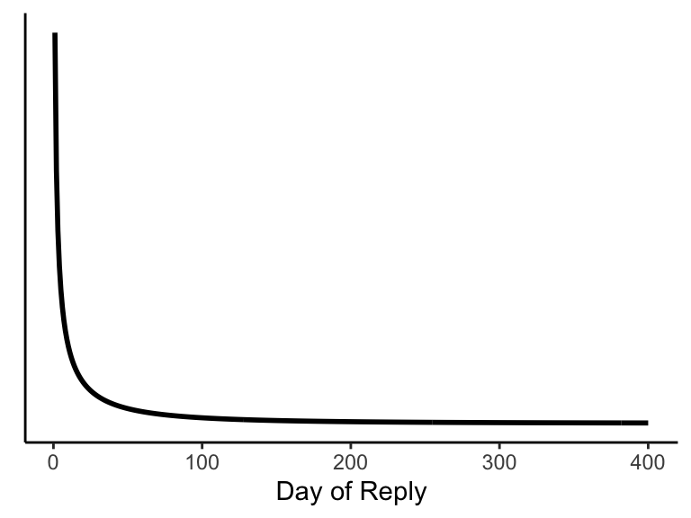
What about this likelihood on the hypothesis that the professor does eventually reply? If we were serious about this, we might dig through our emails to see how long it took to receive replies from various professors. But we don’t have time for that, so let’s instead imagine that the distribution of response times follows a Weibull distribution with a median wait time of around 10 days. The particular version of this distribution that we chose also has the interesting feature that the longer you’ve waited for a reply, the longer you can expect to wait going forward (provided you get an eventual reply). We show this distribution below.
The plot above shows us the probability of receiving a reply on a given day. But for the likelihood, we want the probability of not receiving a reply after some number of days. We can get the probability of having received a reply by day \(x\) (i.e., having received a reply on any day up to and including day \(x\)) from the cumulative distribution function of the Weibull distribution. To get the probability of having not received a reply by then, we just subtract this quantity from 1, leaving us with
\[P(x \text{ days w/o reply}|\text{professor eventually responds})=e^{-(x/\lambda)^k},\]
where \(k=\) 0.5 and \(\lambda=\) 21.
Now to get our rolling posterior,
\[P(\text{professor never responds}|x \text{ days w/o reply}),\]
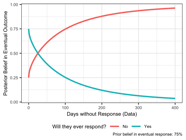
we just need to specify a prior. Let’s assume Ben is initially optimistic: he thinks he’ll receive an eventual reply with probability 0.75 (i.e., \(P(\text{professor never responds})=\) 0.25). The trajectory of his beliefs are shown below. By day 400, he has pretty much given up all hope of ever receiving a reply.
What if we change our hypothesis space slightly to incorporate a new hypothesis? Now instead of simply distinguishing between never receiving a reply and eventually receiving a reply, Ben considers two sub-hypotheses about why he will never receive a reply. In one case, the professor innocuously forgot to respond; in the other case, the professor willfully ignored Ben. In both of these cases, the likelihood is equal to 1 as before (indicating that the professor is guaranteed not to have replied by any day \(x\)), but the priors may be different. In the example below, we show what happens if Ben starts with slightly more credence in the hypothesis that the professor will intentionally ignore him.
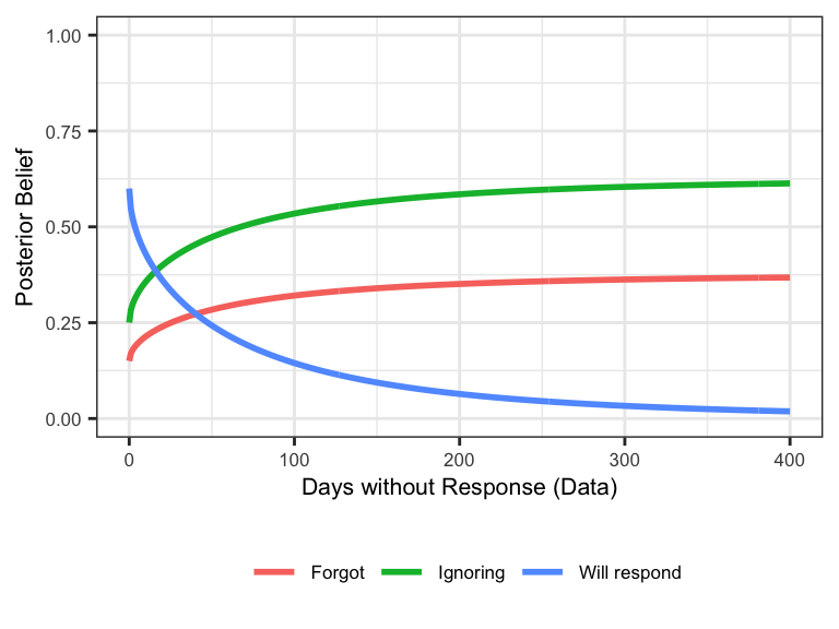
Notice how even though the data can’t distinguish between the “Forgot” and “Ignoring” hypotheses, the priors nevertheless diverge as the “Will respond” hypothesis becomes less plausible. This is an interesting feature of Bayesian reasoning in general: people with slightly different priors and the same evidence can end up drawing starkly different conclusions. Indeed, we could simply flip the red and green lines in the plot above and find that if Ben had assigned slightly more plausibility to the “Forgot” hypothesis relative to “Ignoring,” he would’ve ended up concluding that the professor probably just forgot about his email. How unfortunate.
Linear Regression
What does all of this have to do with statistics? In statistical models like a simple linear regression, we’re rarely modeling an actual process, in the way we might model a coin flip or growth rate of a virus. Instead, we treat some dependent variable as our “data,” and we express this data as a linear function of some independent variable(s) plus a constant, plus noise. This noise is usually assumed to be normally distributed; however, other distributions, such as the Laplace distribution, can also be used. The parameters we want to estimate are therefore the coefficients on the independent variables, the intercept, and the magnitude of the noise (e.g., the standard deviation of the normal distribution).
Let’s consider a simple linear regression with just one independent variable — a model that I’m sure you’re all familiar with. You’re probably used to seeing a regression equation written out like this:
\[\textbf{y} = b_0 + b_1\textbf{x}+\epsilon,\]
where \(b_0\) is the intercept, \(b_1\) is the coefficient on \(x\) and \(\epsilon\) is a normally-distributed noise term with mean of 0. (Note we write \(\textbf{x}\) and \(\textbf{y}\) in bold to indicate that they’re vectors of numbers.) We can equivalently write out this likelihood function as a probability, however, which is easier to connect to the Bayesian machinery:
\[P(D=\textbf{y}|b_0,b_1,\sigma)=\text{Normal}(\textbf{y}|b_0+b_1\textbf{x}, \sigma).\]
More concretely, we model each data point of our dependent variable, \(y_i\) as normally distributed around a mean of \(b_0+b_1x_i\) with standard deviation \(\sigma\). The parameters that maximize the likelihood (i.e., the MLE) of getting all the data points together are identical to the parameter fits from the ordinary least squared (OLS) method.
But remember that, as Bayesians, we don’t want the probability of our data given our parameters, but the probability of our parameters given the data. To compute this, we need to specify priors. When it comes to doing statistics, this is a step that makes a lot of people nervous. Shouldn’t our statistical inference be “objective” and avoid “subjective” priors? Why couldn’t I pick outrageous priors to guarantee that I’ll get the results I want? We’ll have more to say about this when we go through some examples with the brms package, but in general, reasonably specified priors will shrink the estimates relative to OLS, not enlarge them. Let’s see this with an example.
Does need for cognition impact shower preferences?
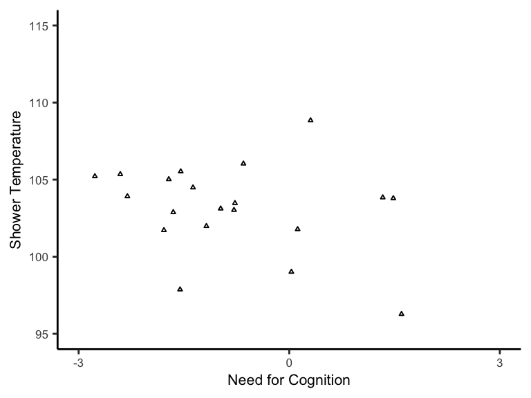
In the glory days of social psychology, it was common to theorize about all sorts of wild correlations between psychological and behavioral variables. Researchers would test their hypothesizes with tiny sample sizes. Let’s consider a silly hypothetical example, where a researcher is interested in the relationship between need for cognition (NFC) and preferred shower temperature (in Fahrenheit).
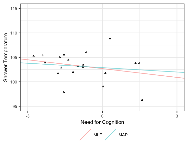
Suppose this was before the days of Mechanical Turk, so the researcher was only able to collect a measly 20 data points. The results are plotted below.
To analyze this data in the Bayesian way, we need to pick priors for the intercept (\(b_0\)) and slope (\(b_1\)). We also technically need to pick a prior for the noise (\(\sigma\)), but for the sake of illustration, we’re going to fix that at 3, which happens to be the true standard deviation used to simulate this data.
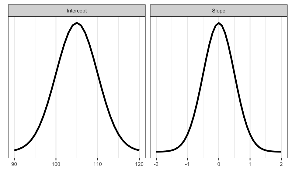
As mentioned above, the prior you choose can cause controversy, so it’s a good idea to simulate data from different priors to make sure the results seem realistic. (We’ll show you how to do this later.) For now, we’ve chosen a normally distributed prior centered at 105 degrees for the intercept, since Google says that’s the average shower temperature; and we’ve chosen a normally distributed prior centered at 0 for the slope.
Why does it make sense to choose 0 for the prior on slope if we have a specific hypothesis that the slope will be positive (or negative)? Well, think about the prior that a skeptic might have. Even if you favor a particular nonzero value of the slope, you need to convince this skeptic (or reviewer) that she should believe that your effect is real. So we almost always center the prior on 0. Note that for both prior distributions, we also limit the spread of the values for good reason. Given what we know, it’s highly implausible that we’d find an average preference for shower temperature below 90 or above 120 degrees, so our model should be suspicious of such extreme values. It’s also implausible that there would be a super strong relationship between NFC and shower temperature in either direction. If there were, we’d almost certainly know about it already. These priors are plotted below.
What about the likelihood? We defined this abstractly above, but let’s be more concrete about how we would calculate it in this case. First of all, it is almost always standard to compute the log of the likelihood, as this is simpler for computers to work with. Then, for each of our data points we can compute the log likelihood as
\[\log(\text{Normal}(y_i|b_0+b_1x_i, \sigma)).\]
The joint log likelihood of all of our data together is just the log of the product of each individual probability, or equivalently, the sum of the logs2:
\[\log(P(D=\textbf{y}|b_0,b_1,\sigma=3))=\sum_i\log(\text{Normal}(y_i|b_0+b_1x_i, \sigma=3)).\]
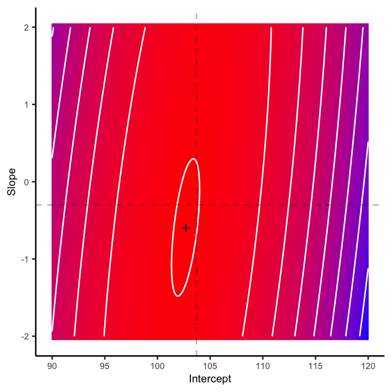
We can visualize this log likelihood as a surface in 2D space, where we independently vary the intercept (\(b_0\)) and slope (\(b_1\)). Redder colors indicate higher log likelihood, and the small black cross is the maximum likelihood estimate. The intersection of the dashed lines is the true combination of parameters that generated our data.
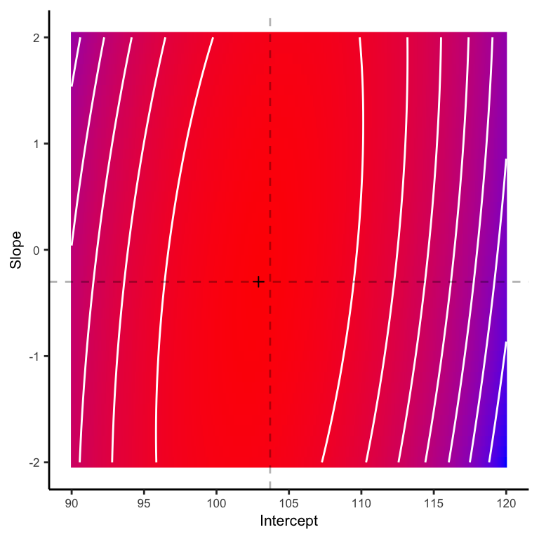
This does a reasonable job, but how does it compare to the (log) posterior estimates? As you can see below, the MAP estimate, indicated by the small cross, is substantially closer to the target.
We can also plot the MLE and MAP estimates as lines fitted to the data. It’s apparent that the MAP estimate is more skeptical than the MLE of there being an effect, as indicated by the shallower slope. This makes sense given the skepticism that we built in to our prior.
It turns out that regression models that build in this skepticism generally make better out-of-sample predictions than those that use standard MLE/OLS. In fact, the MAP estimate from the Bayesian regression we just performed is equivalent to what we would have gotten from a technique in machine learning called ridge regression. So whether or not you’re explicitly using Bayesian statistics, you’re incorporating its logic.
General linear models
We have just covered a simple version of Bayesian linear regression. But this machinery has the power to do much more. In fact, we can import the general linear model from classic statistics into the Bayesian framework without any fuss. For example, we can model count variables with a Poisson distribution and binary variables with a Bernoulli distribution. As in the classic framework, we then need to translate the unbounded predictions from the regression equation into positive values (in the case of count data) or probabilities (in the case of binary data) via log and logit link functions. Just remember to specify your priors.
Additional Resources
We highly recommend checking out Richard McElreath’s Statistical Rethinking textbook, with accompanying videos. Solomon Kurz has also provided a brilliant adaptation of the book that uses the tidyverse and brms R packages.
Because the beta distribution assigns a value to the entire continuous range between 0 and 1, the probability of any particular value of \(p\) is technically 0. However, it is easy to sample a set of discrete \(p\) values and turn them into probabilities by simply recording the height of the function at those points and then normalizing each point so they sum to 1 — a technique known as “grid approximation.”↩︎
This is the version that’s easier for computers to work with, so you should always use it.↩︎