The Pólya urn model of belief

It’s common for modelers to want to estimate uncertainty over fractions or probabilities. For example, we might want to estimate the fraction of people who support a political candidate or the propensity for someone to cooperate. In these cases and many more, we often use a beta distribution (or Dirichlet distribution in the case of more than two categories) to model the plausibility of fractions or probabilities. But why? The following physical analogy to sampling balls from an urn may provide helpful motivation.¹

Imagine there’s an urn in front of you that consists of some mixture of white and black balls. Without knowing how many balls are in the urn, you want to estimate the fraction of the balls that are black. (Suppose that this urn is not constrained by geometry, so it’s possible for it to contain any number of balls.) You can take a few draws from the urn, each time observing the color you draw and then placing the ball back in. But your data is limited; hence, you want to be able to represent your uncertainty over the true proportion of black balls.

This is a daunting problem. Prior to taking samples, all you knew is that the urn contains at least one white ball and at least one black ball. And you’re only allowed to observe a few samples from the urn of unknown size. In theory, then, the urn could contain any fraction of black balls between (but not including) 0 and 1. Nevertheless, let’s see whether we can specify a reasonable procedure for spreading your belief across this infinite space of possible fractions.

Even though we’ve specified that you cannot sample from the urn indefinitely, let’s consider what would happen if you could. After each draw, you could make a note of the color of the ball you drew. You could do this by ‘placing’ a duplicate of this sampled ball into a virtual urn in your imagination. So if you first pull a black ball from the real urn, you place a black ball in your virtual urn, return the real black ball to the real urn, sample from the real urn again, and so on. It doesn’t matter what composition of balls your virtual urn starts with; eventually, this virtual urn will come to resemble the true urn, and you will get an accurate picture of the fraction of balls in the true urn that are black.

Then again, in the absence of other information, you wouldn’t want to initialize your virtual urn with a bunch of virtual balls that you never sampled. Although these initial balls would become irrelevant in the long run, they could reduce the rate at which you converge on the true proportion of black balls in your virtual urn. For example, if you initialized your virtual urn with 3 white balls and 1000 black balls, but the true urn had 15% black balls, you would have to collect a lot of data before your virtual urn would come to resemble the true urn.

How, then, should you initialize your virtual urn? We’ll come back to this question. But as a start, you can reason as follows: Since, prior to sampling any balls from the real urn, all you know is that there is at least one ball of each color, you should initialize your virtual urn with just one white ball and one black ball. This way, your virtual urn will not be biased by some arbitrary starting point.

Now you take a few draws from the real urn and put the appropriately colored balls into your virtual urn. For example, suppose you’ve sampled 6 white balls and 2 black balls, so your virtual urn is filled with 7 white balls and 3 black balls. You stop sampling. We want to know what the current state of your virtual urn tells you about the likely composition of the real urn. For example, how likely is it that the urn is 20% black as opposed to 80% black? In theory, we want to assess the plausibility of any possible fraction of black balls.

Here’s the key insight. Your virtual urn represents your state of belief about what’s in the real urn. So, if you can’t continue sampling from the real urn, you can instead ‘sample’ from the virtual urn. That is, you can use the virtual urn both to represent your current belief about the real urn and to generate hypothetical data from the real urn.

This isn’t a perfect substitute for sampling real data, of course. With only 10 balls in the virtual urn, you may have sampled an unrepresentative set of balls from the real urn. Furthermore, unlike in the real world where there’s a ground truth about what emerges from the urn, you can only simulate what might happen in different possible worlds if you were to sample from the virtual urn as if it were the real urn.

Let’s consider what might happen in one possible world. We imagined that you stopped sampling from the real urn with 7 white balls and 3 black balls in your virtual urn. You will now sample from the virtual urn as a proxy for the real urn. You thus have a 70% chance of drawing a white ball and a 30% chance of drawing a black ball. Let’s say in this possible world your ‘sample’ from the virtual urn turns up a white ball. You now come to believe that the true urn contains more white balls than you expected. In doing so, you place a new white ball into your virtual urn to represent this change in your belief, just as you did when you sampled from the real urn. Now your virtual urn has 8 white balls and 3 black balls. You sample again and get another white ball. You update your belief by putting another white ball into the virtual urn, leaving you with 9 white balls and 3 black balls. And so on.

In general, to simulate one possible long-run outcome of sampling from the true urn, you can implement the following algorithm over many iterations:

1. Take a ‘draw’ from the virtual urn and observe the color of the sampled ball.
2. Put the sampled ball back into the virtual urn along with a duplicate of that ball.
3. Repeat steps 1 & 2 for the updated virtual urn.

This is known as a Pólya urn scheme, named after the mathematician George Pólya who came up with the model. The process is used as a metaphor for dynamics in which a small initial advantage can strengthen over time, as each time you sample a given colored ball, it becomes more likely for you to sample that color again. Many phenomena in the real world work this way (e.g., the “rich getting richer” by investing their disposable income in the stock market and so on), but so does belief. For example, as we encounter more people who support a given candidate, we should come to believe that it’s more likely that the next people we encounter will also support that candidate.

Now we’ve only considered what would happen if we ran this algorithm in one possible world. But to get an accurate sense of how our beliefs about the real urn should be distributed across different possible fractions of black balls, we need to simulate this whole procedure from the beginning many more times. Fortunately, our computers can do this efficiently. Let’s first write a simple R function to simulate one possible long-run trajectory of sampling from the virtual urn for an arbitrary number of draws (n_draws). Then we can run this simulation 10,000 times to get a distribution of our belief about the real urn’s composition.

# Simulate virtual sampling from n_draws, 
# starting with k out of N black balls
simulate_virtual_sampling <- function(n_draws, k, N) {
  for (i in seq_len(n_draws)) {
    d <- rbinom(1, 1, k / N) # draw a ball
    k <- k + d # update count of black balls
    N <- N + 1 # increment total number of balls
  }
  k / N # return final fraction of black balls
}

# Run 10000 simulations with 10000 draws each
# (Run in parallel with the furrr package to speed things up)
library(furrr)
n_sims <- 10000
n_draws <- 10000
k <- 3; N <- 10 # start with 3 out of 10 black balls

set.seed(24)
plan("multisession")
sims <- future_map_dbl(
  seq_len(n_sims), 
  ~simulate_virtual_sampling(n_draws, k, N),
  .options = furrr_options(seed = TRUE)
)

# Plot the distribution of results
library(ggplot2)
ggplot() + 
  geom_histogram(
    aes(sims, after_stat(density)), binwidth = .025,
    fill = "darkblue", color = "white", alpha = 0.5
  ) +
  geom_line(
    aes(
      x = seq(0.01, 0.99, 0.01),
      y = dbeta(seq(0.01, 0.99, 0.01), k, N - k)
    ),
    linetype = "dashed", color = "black", linewidth = 1.5
  ) +
  xlab(
    paste(
      "Fraction of Black Balls after", n_draws, "Draws"
    )
  ) +
  scale_y_continuous(element_blank(), breaks = NULL) +
  coord_cartesian(xlim = c(0, 1)) +
  theme_classic() +
  theme(axis.line.y = element_blank())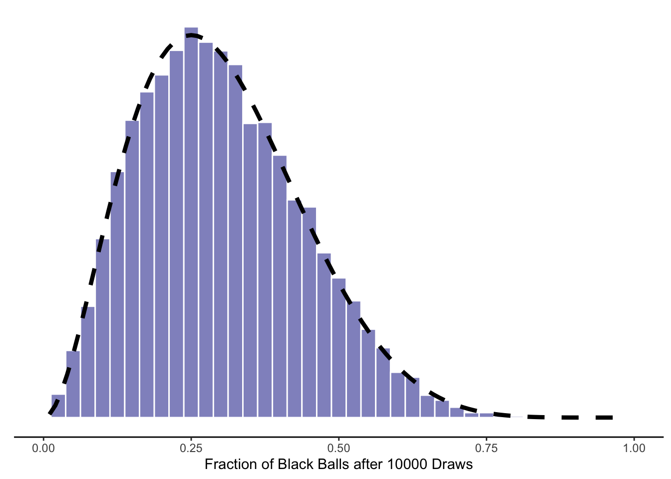

As we’d expect based on your starting point of more white balls than black balls, most of these simulations end up with a majority of white balls. Yet we also have a fair amount of uncertainty, given that you started with only a small number of balls in your virtual urn.

What would happen if we approached the limit of infinite simulations, each run for infinite time? We’d observe the distribution shown with the smooth dashed line — the beta distribution. This distribution takes two parameters, which conveniently correspond to the starting numbers of black (3) and white (7) balls in your virtual urn. If we wanted to consider other possible starting points, all we’d need to do is change these values in the code above.

Given this, if we want to represent our uncertainty over some proportion that can be analogized as an urn, we don’t need to bother with simulations; we can simply query the beta distribution with the relevant “pseudocounts” from our virtual urn.² Moreover, this analogy works for more than two colors. We can represent an urn with an arbitrary number of colored balls with a generalization of the beta distribution known as the Dirichlet distribution. In this case, the Pólya scheme will generate a distribution over ordered sets of probabilities that sum to one. Each sample from this distribution corresponds to a possible long-run fraction of each color (e.g., 22% red, 35% green, 45% blue). This proves to be extremely useful for modeling categories, decisions, and even ordinal variables in linear regression.

One final point. Earlier, we noted that it seemed to make sense, in your state of pure ignorance, to initialize your virtual urn with 1 black and 1 white ball, since all you knew at the time was that the urn contained at least one ball of each color. It turns out that the beta distribution with parameters (1, 1) is just a uniform distribution over all possible fractions between (but not including) 0 and 1. This makes sense: in a state of ignorance, you should believe that any fraction of black balls (other than 0 and 1) is equally plausible.³

In short, the beta distribution, and its generalization to more than two categories, is not simply a mathematically convenient way to capture uncertainty over fractions or probabilities. It is the limiting distribution of a physical process that we expect to converge on the truth.