Imagine you’re a juror in a criminal trial in which the defendant, John, is alleged to have murdered his former boss. The prosecution introduces several types of evidence to bolster their case. One of the strongest pieces of evidence is matching DNA from a stray hair left at the crime scene. Suppose this kind of test only returns a false positive 1 in every 10,000 cases and never returns a false negative. In other words, if we make the simplifying assumption that the presence of John’s hair entails that John is the murdered, then the probability of observing this evidence (\(E\)) if John is the murderer (\(H\)) is 10,000 times greater than the probability of observing this evidence if John is not the murderer (\(\neg H\)). That is,
\[P(E \mid H) = 1 \text{ and } P(E \mid \neg H) = 10^{-4}.\]
What would be a reasonable way to express the strength of this evidence in favor of our hypothesis that John is the murderer?
For starters, we want the evidence to speak for itself. Its strength shouldn’t depend on our prior belief about whether John is the murderer — although it should be sensitive to our beliefs about the relationship between the hypothesis and the data we observe, such as what the exact false positive rate of the DNA test is. In other words, the strength of evidence should only depend on the two conditional probabilities above.
Second, if some observation is equally likely to occur whether or not the hypothesis is true, then this ‘data’ provides zero evidence in favor (or against) our hypothesis. For example, the fact that John was wearing shoes on the day of the murder provides no evidence about his likelihood of being a murderer. On the other hand, the strongest form of evidence in favor of a hypothesis is evidence that’s impossible to arise if the hypothesis is false (regardless of how likely it is to arise when the hypothesis is true). If the DNA test in the trial had a 0% false-positive rate (which would never happen in real life!), then we would learn with certainty that John is the murderer. There’s no amount of evidence stronger than this.
Lastly, since our hypothesis can take on only two values (either John is the murderer or he’s not the murderer), it stands to reason that any evidence for our hypothesis should be matched by an equal amount of negative evidence against this hypothesis, and vice versa.
Putting this all together, there’s a simple mathematical function that satisfies all of these desiderata — the log of the ratio of our two conditional probabilities:
\[ \log(\frac{P(E \mid H)}{P(E \mid \neg H)}). \]
If the two probabilities are equal, this function returns 0; if \(P(E \mid \neg H) = 0\), it returns infinity; and flipping the numerator and denominator to represent evidence against the hypothesis returns the negative of the original value.
This is true no matter what base we use for the logarithm. Perhaps you like to think in base 2 (“evidential bits”) or, if you’re weird like Jaynes, base 10 (which, when multiplied by 10, yields “evidential decibels”). If we express our DNA evidence in decibels, we get a whopping 40 decibels of evidence pointing to John as the murderer.
Two ways of capturing the evidence
Before thinking about new evidence, let’s consider how to represent uncertainty in our hypothesis that John is the murderer. There are (i) probabilities, which range from 0 to 1, and (ii) log odds, which can take on any real number.1 There’s a one-to-one mapping between these quantities. The logit function maps probabilities to log odds:
\[\log(o)=\text{logit}(p) = \log(\frac{p}{1-p}).\]
And the inverse of this function, commonly known as the logistic function, transforms log odds back to probabilities:
\[p=\text{logit}^{-1}(\log(o)) = \frac{1}{1 + e^{-\log(o)}}.\]
If you’re a psychologist like me, you probably learned about the logit function and its inverse when learning about logistic regression or general linear models. These functions give us a convenient method to translate between unbounded predictions from a linear model and bounded probabilities for a binary outcome variable. But these functions turn out to play a pivotal role in Bayesian reasoning, as well, and are intimately tied up with our definition of evidence.
Let’s see how. Bayes’ rule is typically expressed in terms of a probability that a hypothesis is true, given some new evidence:
\[ P(H \mid E) = \frac{P(H)P(E \mid H)}{P(E)}. \]
But we can alternatively express our new posterior belief in log odds:
\[ \log(\frac{P(H \mid E)}{P(\neg H \mid E)}) = \log(\frac{P(H)}{1-P(H)}) + \log(\frac{P(E \mid H)}{P(E \mid \neg H)}). \]
That term on the far right should look familiar — it’s just the strength of the evidence!2 In other words, if we represent our belief in the unbounded space of log odds, Bayes’ rule tells us that a fixed amount of evidence should move our belief a fixed amount, regardless of our prior belief. Or, put slightly differently, two people who start with different prior beliefs and are then exposed to the same evidence will maintain a fixed distance between the log odds of their posterior beliefs. This is, thus, a particularly useful way of modeling people’s beliefs when different people may start with different priors but are exposed to the same evidence.3
On the other hand, there are many cases in which we don’t want to think of prior belief as independent of evidence strength. When we need to make decisions on the basis of our beliefs, the usefulness of acquiring a fixed amount of evidence can vary considerably based on what we already believe.
Consider two versions of the murder trial from earlier. In one case, the jurors have already watched a clear surveillance video of John shooting his boss; in the other case, they’ve only heard weak circumstantial evidence linking John to the murder. How will these two juries react to the same 40-decibel DNA evidence? The first jury likely already strongly believed, beyond a reasonable doubt, that John murdered his boss, and therefore the DNA evidence is irrelevant to their verdict. To the second jury, though, this DNA evidence is likely to make the difference between “not guilty” and “guilty.”4
Bridging the two representations
So the log odds format and the probability format of representing belief have different advantages. To simplify matters slightly, while a fixed distance in log-odds space is a measure of evidential strength, a fixed distance in probability space is a measure of a person’s responsiveness to evidence (e.g., for decision-making). In probability space, weak evidence for someone who is very unsure of a hypothesis can have the same or greater impact as strong evidence for someone who is very sure of this hypothesis.
How can we model the ‘impact’ of a fixed amount of evidence? As discussed, log odds are converted to probabilities via the logistic (inverse logit) function:
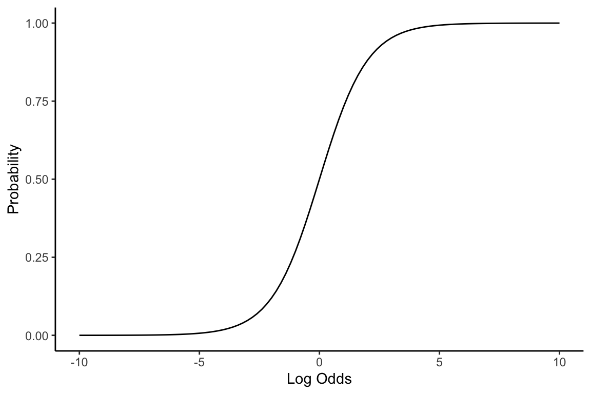
A fixed change on the x-axis thus represents a constant amount of evidence. The slope of this line represents our sensitivity to evidence, which varies depending on where our prior belief is. When the log odds of the prior are near 0 (i.e., probability of 0.5), we’re most sensitive to evidence; when they are far from 0 in either direction (i.e., probability close to 0 or 1), we’re least sensitive to the same amount of evidence.
We can use calculus to explore what happens as we shrink this fixed amount of evidence down to an infinitesimally small number, \(\epsilon\). The slope of the logistic function at a given prior log odds will then be given by the derivative of this function. In other words, the derivative of the logistic function captures how we (rational Bayesians) will react, in probability space, to a marginal amount of evidence5:
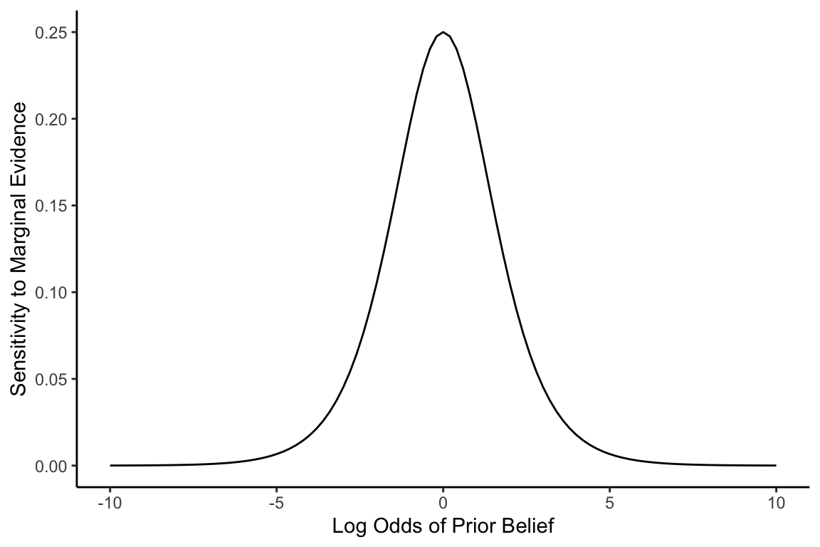
What is this mysterious function? It’s actually simpler than it looks. The derivative of a logistic function is just that function multiplied by one minus itself:
\[ \frac{d}{dx}\text{logit}^{-1}(x)=\text{logit}^{-1}(x)(1-\text{logit}^{-1}(x)). \]
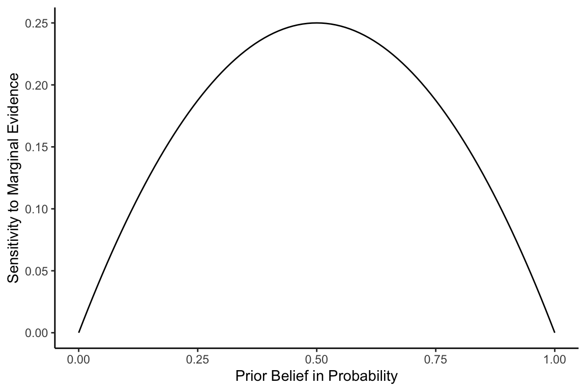
Moreover, recall that if \(x\) is a prior belief in log odds, then \(\text{logit}^{-1}(x)\) gives the prior belief in probability, \(P(H)\). In other words, by changing the x-axis in the above plot to prior belief in probability space, the sensitivity to marginal evidence becomes \(P(H)(1-P(H))\):
The missing link
Why would our sensitivity to evidence be captured by the product of our prior probability that the hypothesis is true, \(P(H)\), and our prior probability that the hypothesis is false, \(1 - P(H)\)?
Clearly, the answer has something to do with uncertainty, but how should we formalize this concept? An information theorist represents uncertainty in terms of entropy, or our expected ‘surprise’ from learning that our hypothesis is true or false. Just like the function we drew above, the entropy of a binary variable is maximized when the probability is 0.5 (1 bit of information) and minimized when the probability is 0 or 1 (0 bits of information). But, surprisingly, it’s not equal to \(P(H)(1-P(H))\)!6
Maybe we can represent uncertainty more simply. Intuitively, our belief in probability space is constrained by the amount we maximally could move when presented with conclusive evidence for or against our hypothesis. The hypothetical jurors who were presented with strong DNA evidence in support of John’s guilt after they had already seen the murder on video did not move their belief much because their prior belief was already very close to 1. Of course, it was also possible for them to receive evidence of his innocence (e.g., later learning that the video was fabricated by the true murderer to lead the jury astray). But, if the jurors had well-calibrated beliefs, this should have been extremely unlikely.
To formalize this concept of ‘maximal possible movement’, we can consider how much we, with our prior belief of \(P(H)\), would move if we definitively learned that our hypothesis is true vs. if we definitively learned that our hypothesis is false. Since our belief is bounded at 0 and 1, the former is equal to \(1-P(H)\), and the latter is equal to \(P(H)\). To capture our expected belief update in the face of conclusive evidence for or against the hypothesis, we just take a weighted average of these two distances. We believe we’d learn the hypothesis is true with probability \(P(H)\) and learn it’s false with probability \(1-P(H)\). Hence, our expected belief update from conclusive evidence is
\[ P(H)(1-P(H))+(1-P(H))P(H)=2P(H)(1-P(H)). \]
For all intents and purposes, this is the expression we’re looking for. It tells us that the amount that a marginal amount of evidence moves our belief scales with the amount we would expect to move from maximal evidence.
But where’s that pesky factor of two coming from? Although it’s irrelevant if we’re just thinking about proportionality, is there a way to get rid of it? Let’s try a common statistical trick: squaring the distances from above. That is, rather than calculate our prior’s expected absolute distance from 0 and 1, we solve for
\[ P(H)(1-P(H))^2 + (1-P(H))P(H)^2. \]
This quantity — also known as the variance of a Bernoulli random variable — reduces to
\[ P(H)-2P(H)^2+P(H)^3+P(H)^2-P(H)^3=P(H)(1-P(H)). \]
And there you have it! Our sensitivity to a fixed amount of marginal evidence is identical to our expected squared movement from infinitely strong evidence. Or, if you prefer, it’s the variance of the sequence of 0s and 1s we would draw if we were to sample 1s in proportion to our prior belief.
But if you’re just as puzzled as me about why we would square the distances from our prior belief, rest assured that the non-squared version works just as well.
There are also (non-logged) odds, which range from 0 to infinity, but I won’t be touching those.↩︎
You might also know this as the log likelihood ratio.↩︎
For example, in psychology and neuroscience, the drift diffusion model represents belief in a binary hypothesis in log-odds space for this reason.↩︎
We can’t really formalize the concept of “usefulness” without bringing in utilities, which vary from context to context. But, all else equal, a fixed amount of evidence will be most likely to change our decision when we were most uncertain before receiving this evidence.↩︎
Because the logistic function is the cumulative density function of a standard logistic distribution (i.e., a logistic distribution with a mean of 0 and a variance of \(\pi^2/3\)), the derivative of this function is just the probability density function of a standard logistic distribution.↩︎
There is a similarly deep connection between the entropy of a Bernoulli random variable (as measured in bits) and the logit function (using log base 2), however. The derivative of the binary entropy function is the negative log (base 2) odds. This captures the fact that expected surprise is relatively flat near its maximum at probability of 0.5, but increases rapidly as you move from absolute certainty (at probabilities of 0 or 1) to near certainty.↩︎